Wavelet Analysis

clc;clear all;close all;

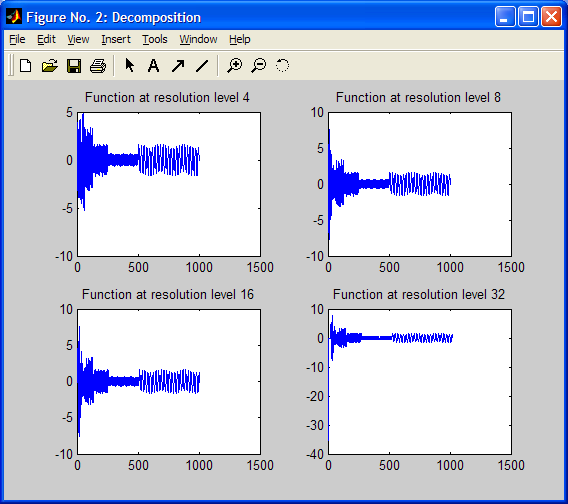
% The function is displayed at different resolution levels, j = 4, 8, 16, 32
% The current extension mode is zero-padding (see dwtmode).
% Load original one-dimensional signal.

load sumsin;
s = sumsin;

% Perform decomposition at level 3 of s using db1.
% WAVEDEC –> Multi-level 1-D wavelet decomposition.
% WAVEDEC performs a multilevel 1-D wavelet analysis using either a specific wavelet
% ‘wname’ or a specific set of wavelet decomposition filters.
%  [C,L] = WAVEDEC(X,N,’wname’) returns the wavelet
%  decomposition of the signal X at level N, using ‘wname’.

figure (‘Name’,’Input 1-D Signusoidal Signal’);
plot(s);

figure (‘Name’,’Decomposition’);

% ‘bior1.1’ –> Biorthogonal wavelet filter

[c,l] = wavedec(s,4,’bior1.1′);
subplot(2,2,1);
plot(c);
title(‘Function at resolution level 4’);

[c,l] = wavedec(s,8,’bior1.1′);
subplot(2,2,2);
plot(c);
title(‘Function at resolution level 8’);
[c,l] = wavedec(s,16,’bior1.1′);

subplot(2,2,3);
plot(c);
title(‘Function at resolution level 16’);

[c,l] = wavedec(s,32,’bior1.1′);
subplot(2,2,4);
plot(c);
title(‘Function at resolution level 32’);

% % DWT –> Single-level discrete 1-D wavelet transform
% % [CA,CD] = DWT(X,’wname’) computes the approximation
% % coefficients vector CA and detail coefficients vector CD

% [CA,CD] = DWT(s,’bior1.1′);
% figure(‘Name’,’Approximate Coeeficients’), plot(CA);
% figure(‘Name’,’Actual/Detail Coeeficients’), plot(CD);