MSc Computer Science Image Processing Practical No. 1
Index of all Practicals ~ Click Here
Code:– Image_enh_spat_dom.m
% ******** CONTRAST STRETCHING ********
f = imread(‘moon.tif’);
subplot(2,2,1);
imshow(f);
title(‘Original Image’);
subplot(2,2,2);
imhist(f);
title(‘Histogram’);
figure;
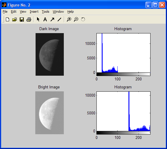
g = imadjust(f,[0 1],[0.1 0.4]);
subplot(2,2,1);
imshow(g);
title(‘Dark Image’);
subplot(2,2,2);
imhist(g);
title(‘Histogram’);
g = imadjust(f,[0 1],[0.6 1.0]);
subplot(2,2,3);
imshow(g);
title(‘Bright Image’);
subplot(2,2,4);
imhist(g);
title(‘Histogram’);
figure;
g = imadjust(f,[0 1],[0.4 0.7]);
subplot(2,2,1);
imshow(g);
title(‘Low-contrast image’);
subplot(2,2,2);
imhist(g);
title(‘Histogram’);
g = imadjust(f,[0 1],[0.1 1.0]);
subplot(2,2,3);
imshow(g);
title(‘High-contrast image’);
subplot(2,2,4);
imhist(g);
title(‘Histogram’);
figure;
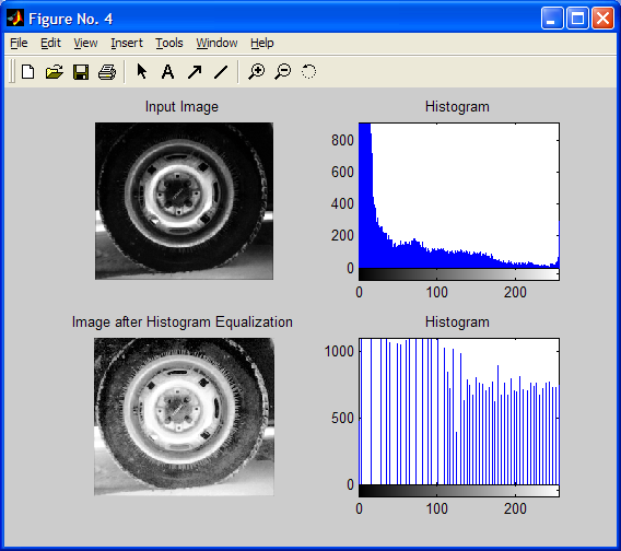
f = imread(‘tire.tif’);
g = histeq(f);
title(‘Histogram’);
% The process of adjusting intensity values can be done automatically by the histeq function.
% It involves transforming the intensity values so that the histogram
% of the output image approximately matches a specified histogram.
subplot(2,2,1);
imshow(f);
title(‘Input Image’);
subplot(2,2,2);
imhist(f);
title(‘Histogram’);
subplot(2,2,3);
imshow(g);
title(‘Image after Histogram Equalization’);
subplot(2,2,4);
imhist(g);
title(‘Histogram’);
OR
f=imread(‘tire.tif’);
g=double(f);
[row col]=size(g);
h=zeros(1,300);
z=zeros(1,300);
c=row*col;
rmax=(max(max(g)));
for x=1:row
for y=1:col
if f(x,y)==0
f(x,y)=1;
end
end
end
for x=1:row
for y=1:col
t=f(x,y);
h(t)=h(t)+1;
end
end
pdf=h/c;
cdf(1)=pdf(1);
for x=2:rmax
cdf(x)=pdf(x)+cdf(x-1);
end
eimg=round(cdf*rmax);
eimg=eimg+1;
for x=1:row
for y=1:col
r=aa(x,y);
b(x,y)=eimg(r);
t=b(x,y);
z(t)=z(t)+1;
end
end
b=b+1;
figure(1);
imshow(uint8(g));
figure(2);
bar(h);
figure(3);
imshow(uint8(b));
figure(4);
bar(z);
figure;
f = imread(‘moon.tif’);
% D –> Noise Density
D = 0.02;
g = imnoise(f,’salt & pepper’,D);
% n = imsubtract(f,g);
subplot(1,2,1);
imshow(g);
title(‘Noisy Image g(x,y)=f(x,y) + n(x,y)’);
avg = filter2(fspecial(‘average’,3),g)/300;
subplot(1,2,2);
imshow(avg);
title(‘Averaging Filter Image’);
f = imread(‘rice.png’);
n = 10;
Wn = 0.2;
mask = fir1(n,Wn);
% This create a mask containing the coefficients of the order n Hamming-windowed filter.
% This is a lowpass, linear phase FIR filter with cutoff frequency Wn.
g = imfilter(f,mask);
figure;
subplot(1,2,1);
imshow(f);
title(‘Original Image’);
subplot(1,2,2);
imshow(g);
title(‘Smoothning Effect due to a given mask’);
Output:-


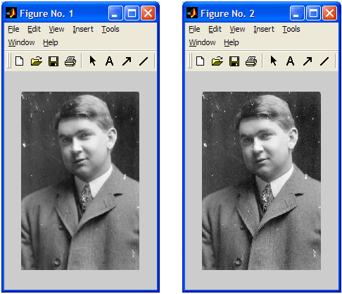
Program Using Formulas
Code:- Pract1_Low.m
clear all;
close all;
a=imread(‘Old Image.jpg’);
r=double(a);
[row col]=size(r);
w=[1 1 1;1 1 1;1 1 1 ]/9;
for x=2:row-1
for y=2:col-1
b(x,y)=r(x-1,y-1)*w(1)+r(x-1,y)*w(2)+r(x-1,y+1)*w(3)+ r(x,y-1)*w(4)+r(x,y)*w(5)+r(x,y+1)*w(6)+r(x+1,y-1)*w(7)+r(x+1,y)*w(8)+r(x+1,y+1)*w(9);
end
end
figure(1);
imshow(uint8(b));
figure(2);
imshow(uint8(r));
Output:-
Code:- Pract1_Gaussian.m
a=imread(‘Ranch house.jpg’);
%r1=double(a);
r2=imnoise(a,’gaussian’);
r=double(r2);
[row col]=size(r);
w=[1 1 1;1 1 1;1 1 1 ]/9;
for x=2:row-1
for y=2:col-1
b(x,y)=r(x-1,y-1)*w(1)+r(x-1,y)*w(2)+r(x-1,y+1)*w(3)+ r(x,y-1)*w(4)+r(x,y)*w(5)+r(x,y+1)*w(6)+r(x+1,y-1)*w(7)+r(x+1,y)*w(8)+r(x+1,y+1)*w(9);
end
end
figure(1);
imshow(uint8(b));
figure(2);
imshow(uint8(r));
Output:-

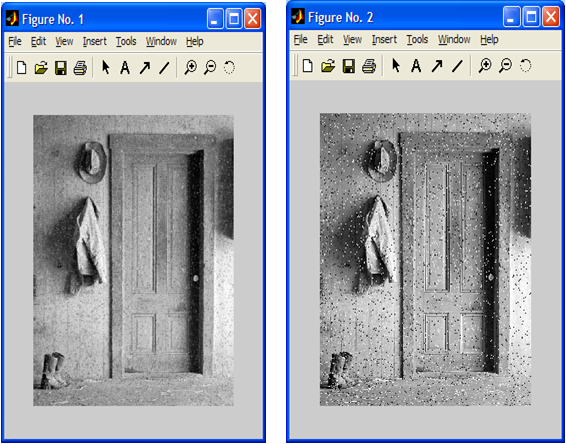
Code:- Pract1_Salt.m
a=imread(‘Ranch house.jpg’);
%r1=double(a);
r2=imnoise(a,’salt & pepper’);
r=double(r2);
[row col]=size(r);
w=[1 1 1;1 1 1;1 1 1 ]/9;
for x=2:row-1
for y=2:col-1
b(x,y)=r(x-1,y-1)*w(1)+r(x-1,y)*w(2)+r(x-1,y+1)*w(3)+ r(x,y-1)*w(4)+r(x,y)*w(5)+r(x,y+1)*w(6)+r(x+1,y-1)*w(7)+r(x+1,y)*w(8)+r(x+1,y+1)*w(9);
end
end
figure(1);
imshow(uint8(b));
figure(2);
imshow(uint8(r));
Output:-
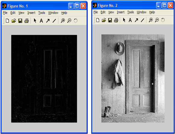
Code:- Pract1_High.m
a=imread(‘Ranch house.jpg’);
r=double(a);
[row col]=size(r);
w=[-1 -1 -1;-1 8 -1;-1 -1 -1 ]/9;
for x=2:row-1
for y=2:col-1
b(x,y)=r(x-1,y-1)*w(1)+r(x-1,y)*w(2)+r(x-1,y+1)*w(3)+ r(x,y-1)*w(4)+r(x,y)*w(5)+r(x,y+1)*w(6)+r(x+1,y-1)*w(7)+r(x+1,y)*w(8)+r(x+1,y+1)*w(9);
end
end
figure(1);
imshow(uint8(b));
figure(2);
imshow(uint8(r));
Output:-
Code:- Pract1_Highm.m
a=imread(‘Ranch house.jpg’);
r=double(a);
[row col]=size(r);
w=[-1 -1 -1;-1 8.9 -1;-1 -1 -1 ];
for x=2:row-1
for y=2:col-1
b(x,y)=r(x-1,y-1)*w(1)+r(x-1,y)*w(2)+r(x-1,y+1)*w(3)+ r(x,y-1)*w(4)+r(x,y)*w(5)+r(x,y+1)*w(6)+r(x+1,y-1)*w(7)+r(x+1,y)*w(8)+r(x+1,y+1)*w(9);
end
end
figure(1);
imshow(uint8(b));
figure(2);
imshow(uint8(r));
Output:-
